Introduction:

In the field of machine learning and data analysis, working with high-dimensional data can often be challenging. Dimensionality reduction techniques like PCA (Principal Component Analysis) and t-SNE (t-Distributed Stochastic Neighbor Embedding) offer effective solutions to this problem. In this blog, we will explore the concepts of PCA and t-SNE, explain their differences, and provide Python code snippets to illustrate their application.

Principal Component Analysis (PCA):

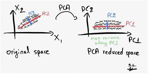
PCA is a widely used linear dimensionality reduction technique that seeks to find a new set of orthogonal axes, called principal components, which capture the maximum variance in the data. The idea behind PCA is to transform the original high-dimensional data into a lower-dimensional space while retaining as much information as possible. Let's consider an example where we have a dataset with three features: height, weight, and age. Using PCA, we can project this data onto a two-dimensional space while preserving the most important characteristics.

Python code snippet for PCA:

from sklearn.decomposition import PCA
from sklearn.manifold import TSNE
from sklearn.datasets import load_iris
import plotly.graph_objects as go

# Load the Iris dataset from scikit-learn
iris = load_iris()
X = iris.data  # The input data matrix
y = iris.target  # The target labels

# Perform PCA with 3 components
pca = PCA(n_components=3)
X_pca = pca.fit_transform(X)


# Create a 3D plot using Plotly for PCA
fig_pca = go.Figure(data=[go.Scatter3d(
    x=X_pca[:, 0],
    y=X_pca[:, 1],
    z=X_pca[:, 2],
    mode='markers',
    marker=dict(
        size=5,
        color=y,
        colorscale='Viridis',
        opacity=0.8
    )
)])
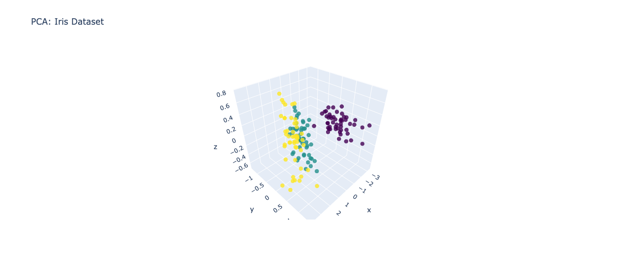
fig_pca.update_layout(title='PCA: Iris Dataset')
fig_pca.show()

t-Distributed Stochastic Neighbor Embedding (t-SNE):

t-SNE is a non-linear dimensionality reduction technique that is particularly useful for visualizing high-dimensional data in a two- or three-dimensional space. Unlike PCA, t-SNE focuses on preserving the local structure of the data rather than the global variance. It accomplishes this by constructing a probability distribution over pairs of high-dimensional points and a similar distribution over the corresponding low-dimensional points. Let's continue with our previous example. Using t-SNE, we can generate a scatter plot that preserves the local structure of the data, making it easier to identify clusters or patterns.

Python code snippet for t-SNE:

from sklearn.decomposition import PCA
from sklearn.manifold import TSNE
from sklearn.datasets import load_iris
import plotly.graph_objects as go

# Load the Iris dataset from scikit-learn
iris = load_iris()
X = iris.data  # The input data matrix
y = iris.target  # The target labels

# Perform t-SNE with 3 components
tsne = TSNE(n_components=3)
X_tsne = tsne.fit_transform(X)

# Create a 3D plot using Plotly for t-SNE
fig_tsne = go.Figure(data=[go.Scatter3d(
    x=X_tsne[:, 0],
    y=X_tsne[:, 1],
    z=X_tsne[:, 2],
    mode='markers',
    marker=dict(
        size=5,
        color=y,
        colorscale='Viridis',
        opacity=0.8
    )
)])

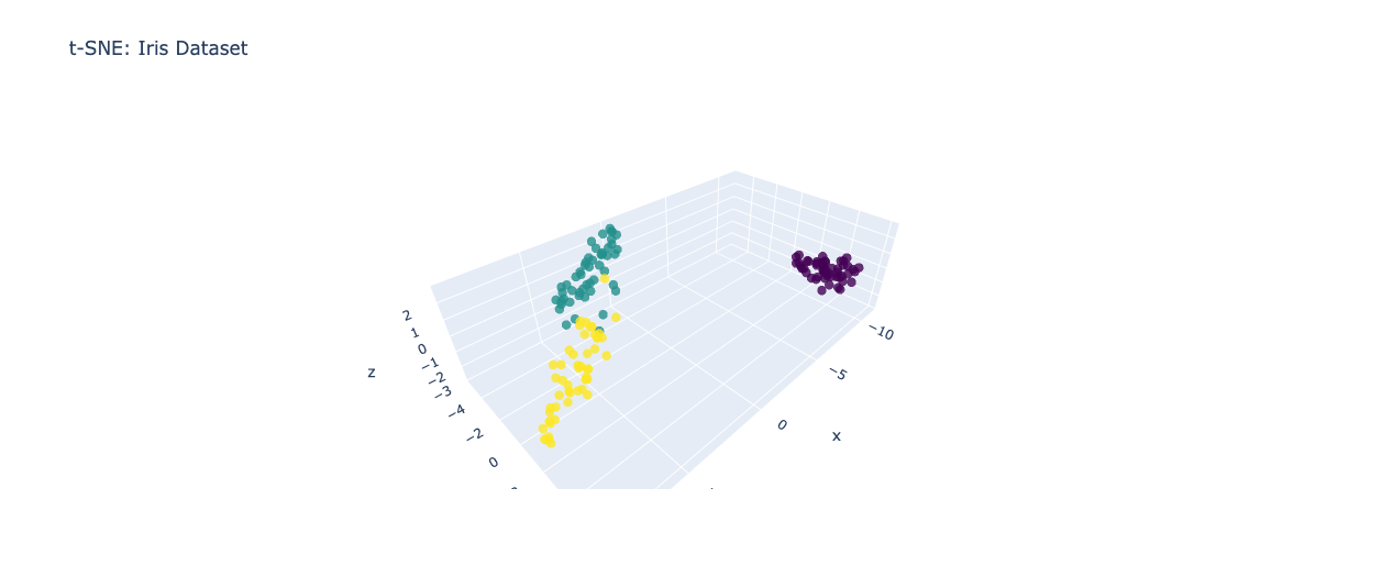
fig_tsne.update_layout(title='t-SNE: Iris Dataset')

fig_tsne.show()

Differences between PCA and t-SNE:

• Linearity vs. Non-linearity: PCA is a linear technique, meaning it looks for linear relationships between variables. t-SNE, on the other hand, is non-linear, allowing it to capture complex patterns that may not be linearly separable.
• Preserved Information: PCA aims to preserve global variance, whereas t-SNE emphasizes the preservation of local structures and clusters.
• Computational Complexity: PCA is computationally efficient and suitable for large datasets, while t-SNE has a higher computational complexity and is more suitable for visualizing smaller datasets.

When to use PCA and t-SNE:

Use PCA when the global variance of the data is important, and you want a computationally efficient dimensionality reduction method. Use t-SNE when you want to visualize the local structures and clusters in your data, especially for small to medium-sized datasets.

Conclusion:

PCA and t-SNE are both valuable dimensionality reduction techniques with distinct characteristics. PCA is useful for capturing global variance efficiently, while t-SNE excels at preserving local structures and enabling effective data visualization. Understanding their differences and knowing when to apply each method can greatly enhance data analysis and machine learning tasks.

Remember to experiment with different techniques and evaluate the results based on your specific dataset and objectives.